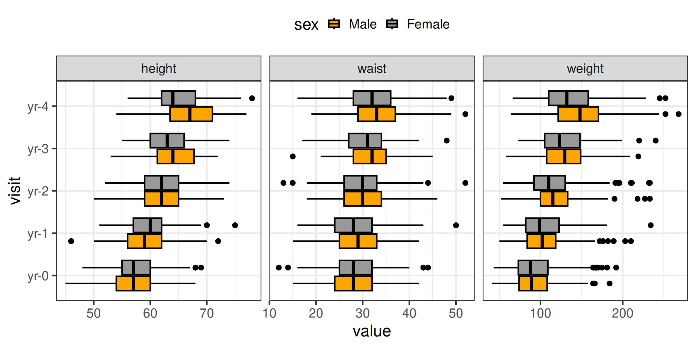
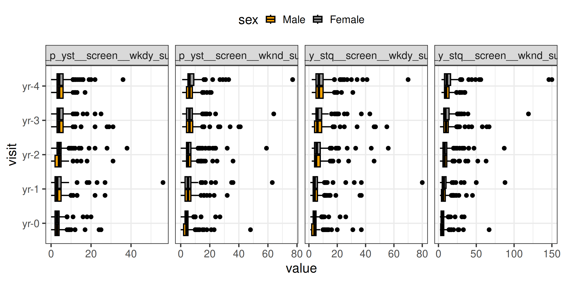
Module 2 built every figure by copying the one before and changing a few lines. That is the right way to discover an analysis. It is the wrong way to keep one. This page takes the Module 2 code and turns it, one step at a time, into a handful of small functions — until the whole session fits in about six lines.
library(dplyr)
Attaching package: 'dplyr'
The following objects are masked from 'package:stats':

    filter, lag
The following objects are masked from 'package:base':

    intersect, setdiff, setequal, union
── Column specification ────────────────────────────────────────────────────────
Delimiter: ","
chr (2): name, label
dbl (2): value, order_level
lgl (1): label_es

ℹ Use `spec()` to retrieve the full column specification for this data.
ℹ Specify the column types or set `show_col_types = FALSE` to quiet this message.
Why bother
Look back at Module 2’s Exercise 1. Its solution is the Q1 facet pipeline with three lines changed. Exercise 2 is the Q2 pipeline with one measure swapped. Two copies, each drifting slightly away from the original — and one real bug that drifted in: Q1 sets the order of sex and Q2 does not, so the colours swap between the two figures.
Copies go wrong in exactly this way. Fix a problem in one and you have to remember every other place it was pasted. A function is a named piece of code you write once and call many times. Fix it once, and every call is fixed.
A common rule of thumb: once you have copied a block of code twice, make it a function.
The anatomy of a function
se <-function(x) {sd(x, na.rm =TRUE) /sqrt(sum(!is.na(x)))}
Four parts:
se — the name, assigned with <- like any other object
function(x) — the arguments: the inputs, and the names they go by inside the function
{ ... } — the body: the code that runs
the return value — whatever the last line of the body produces. No return() needed
That function is the standard error from Module 2 — SD divided by the square root of n — written so it copes with missing values: sum(!is.na(x)) counts only the values that are present. Call it like any built-in function:
se(c(4, 8, 6, NA, 5))
[1] 0.8539126
sub_screen <- data |>group_by(session_id) |>summarise(mean =mean(nt_y_stq__screen__wkdy_sum, na.rm =TRUE),se =se(nt_y_stq__screen__wkdy_sum) )sub_screen
You have been using defaults since Module 1: mean() has na.rm = FALSE unless you say otherwise.
TipYou have met one already
The wrangling deep-dive wrote apply_labels(x, var), which labels any coded variable from the dictionary. Same anatomy: two arguments, a body, and the last line’s value returned.
Functions around dplyr: { }
se() works on a vector. The Module 2 code, though, is pipelines, and the natural next step — passing a column name into a function — fails in a way that confuses everyone the first time:
mean_of <-function(data, var) { data |>summarise(mean =mean(var, na.rm =TRUE))}mean_of(data, ph_y_anthr__height_mean)
Error in `summarise()`:
ℹ In argument: `mean = mean(var, na.rm = TRUE)`.
Caused by error:
! object 'ph_y_anthr__height_mean' not found
Inside a dplyr verb, a bare name like height means “the column called height”. But inside a function, var is just an argument. dplyr looks for a column literally called var, does not find one, and then looks for an ordinary variable instead — and fails.
The fix is to embrace the argument with double braces, { var }. It tells dplyr: “don’t use the word var; use whatever the caller typed in its place.”
mean_of <-function(data, var) { data |>summarise(mean =mean({{ var }}, na.rm =TRUE))}mean_of(data, ph_y_anthr__height_mean)
     mean
1 60.9073
That is the one rule to remember: when an argument is a column name that is passed into a dplyr or ggplot2 function, wrap it in { }.
A summary function
Now the Q2 summary — n, mean, SD and SE per group — as a function. The ... (“dots”) argument collects any number of extra arguments and passes them on, here to group_by(), so the caller can group by as many columns as they like:
summarise_mean_se <-function(data, var, ...) { data |>filter(!is.na({{ var }})) |>group_by(...) |>summarise(n =n(),mean =mean({{ var }}),sd =sd({{ var }}),se = sd /sqrt(n),.groups ="drop" )}data |>summarise_mean_se(nt_y_stq__screen__wkdy_sum, session_id)
One line per summary table, for any variable and any grouping.
Wrap the data preparation
Module 2’s section 3 turned data into sub2: select and rename, round, recode sex, build visit, join the site labels. Here it is in full as the “before” — the same code, minus the glimpse() calls used to peek during the live session:
site_levels is now created inside the function. It exists only while the function runs and cannot clash with anything else in your session — one of the quiet benefits of functions.
Whenever you refactor, check that nothing changed:
identical(format_abcd(data, levels_dict), sub2)
[1] TRUE
identical() compares two objects exactly. TRUE means the function gives the same sub2, value for value, as the original pipeline.
Functions that return plots
A ggplot is an object like any other, so a function can build one and return it. The same { } rule applies inside aes() and inside tidyselect arguments such as select() and pivot_longer(cols = ).
Reusable layer bundles
First, the pieces every Module 2 figure repeated — the theme, the legend position, the colours. A function can return a list() of layers, and ggplot2 adds every item in the list when you + it:
Note the named colour values. c(Male = "orange", ...) ties each colour to a category rather than to a position, so males are orange whatever order the levels are in. That fixes Module 2’s colour-swap bug once, for every figure that uses scale_sex().
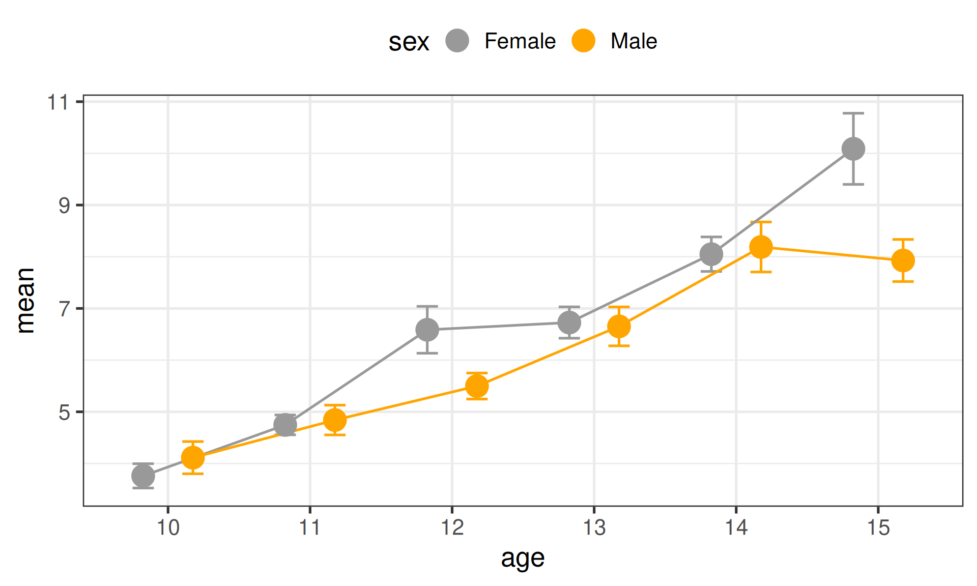
Figure 3: Q2 from Module 2, as a short pipeline of function calls
Males are orange again, as in Q1 — the named colours at work. The legend still lists Female first, because legend order comes from the factor levels, not from the colour names. Add mutate(sex = factor(sex, levels = c("Male", "Female"))) if the order matters.
One small difference from the original: Q2 dropped a row if any of four measures was missing, while summarise_mean_se() only needs the one being summarised. So each group here keeps a few more participants (146 rather than 140 girls at age 10, for instance), and the means shift very slightly. Neither rule is wrong, but a refactor is a good moment to choose one deliberately.
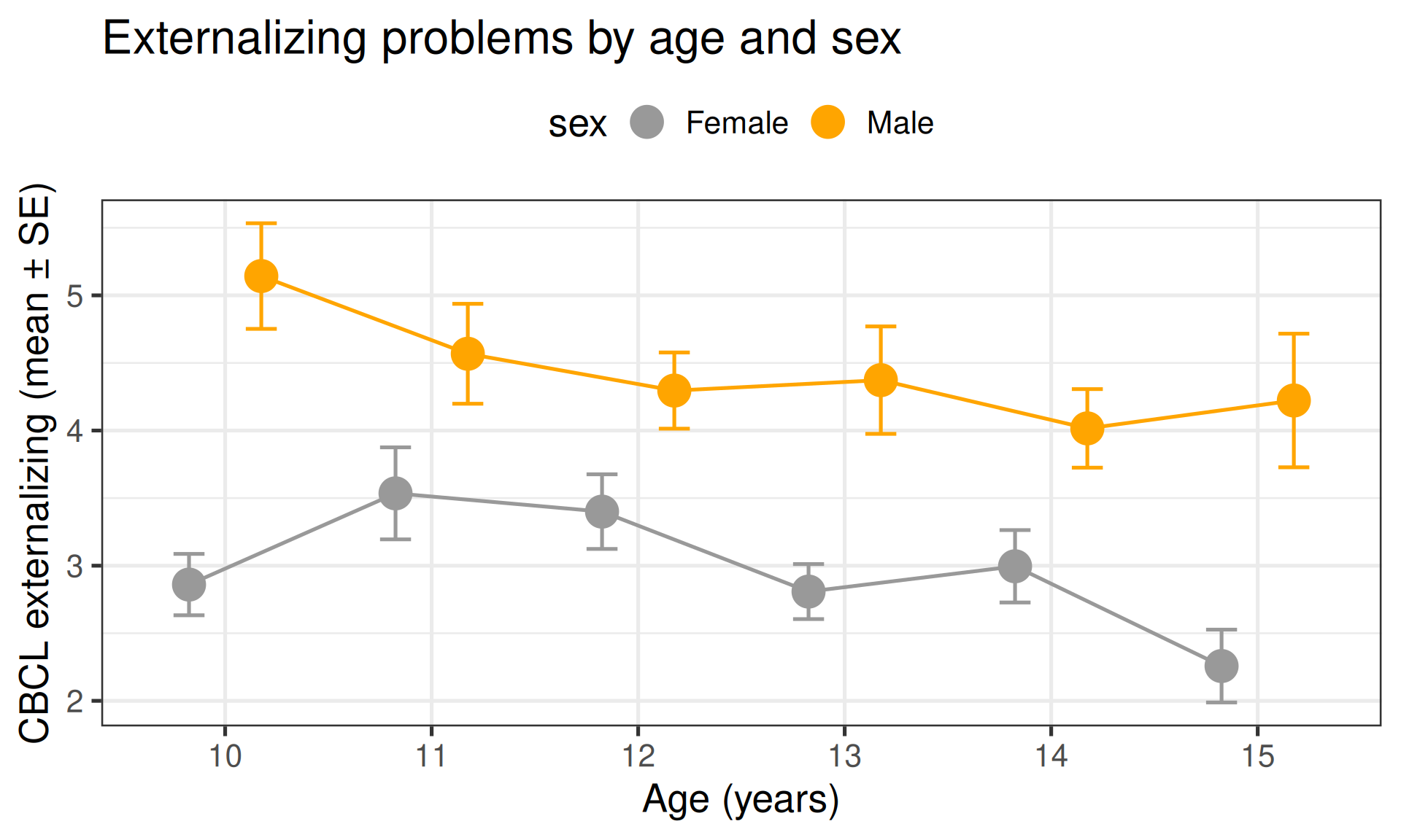
Because the function returns an ordinary ggplot, you can keep adding layers to the result:
sub2 |>filter(age >=10& age <=15) |>mutate(age =factor(age)) |>summarise_mean_se(mh_p_cbcl__synd__ext_sum, age, sex) |>plot_mean_se(age, sex) +labs(x ="Age (years)",y ="CBCL externalizing (mean ± SE)",title ="Externalizing problems by age and sex" )
Figure 4
Putting it together
Everything from Module 2, with the functions defined above:
Each line says what it does, not how. The how lives in one place.
The same plot for many variables
With column names held as text, one more piece of syntax is needed: .data[[name]] means “the column whose name is stored in name”. It works anywhere a bare column name would, including through { }:
lapply() runs the function once for each element of outcomes and returns a list of the results — here, three finished plots. (\(v) is shorthand for function(v).) Look at any one with plots[[2]], or save them all:
for (i inseq_along(plots)) {ggsave(paste0("output/", outcomes[i], ".png"),plot = plots[[i]],width =10, height =6, dpi =300 )}
Adding a fourth outcome is now a one-word change.
Keeping functions in a file
Functions defined in the middle of an analysis script get lost. Put them in their own file in your project — for example R/functions.R — and load them at the top of every script that needs them:
source() runs every line of a file, so the functions are defined and ready to use. The same relative-path rule from Module 1 applies: it works because your RStudio Project sets the working directory.
Failing helpfully
A function used by other people — or by you in three months — should say clearly when it is being misused. Without a check, passing the raw data to plot_boxplots() fails deep inside mutate() with an error about a column called sex. A check at the top turns that into a message the caller can act on:
plot_boxplots <-function(data, cols) {if (!"sex"%in%names(data)) {stop("`data` needs a `sex` column. Run format_abcd() on it first.") } data |>mutate(sex =factor(sex, levels =c("Male", "Female"))) |>select(participant_id, visit, sex, {{ cols }}) |> tidyr::pivot_longer(cols = {{ cols }}, names_to ="what", values_to ="value") |>mutate(visit =paste0("yr-", visit) |>factor()) |>ggplot(aes(x = visit, y = value, fill = sex)) +geom_boxplot(col ="black") +facet_grid(~ what, scales ="free") +coord_flip() +scale_sex() +theme_workshop()}plot_boxplots(data, height:waist)
Error in `plot_boxplots()`:
! `data` needs a `sex` column. Run format_abcd() on it first.
stop() halts the function with your message. The error names the function, says what is wrong, and says what to do about it — the three things a good error message needs.