Module 1: Foundations of R Programming

Biplabendu [ Billu ] Das

This module is for someone who has never used R. By the end of two hours you will have read a real dataset into R, pulled it apart to answer questions about it, dealt with missing values, and made three plots.

We teach R the way most modern R is written: tidyverse style, using the |> pipe. Along the way we point out the bits of plain “base R” notation you need in order to read code you find on the internet.

Before you start

Work through Module 0 first — R and RStudio installed, an RStudio Project open, the packages installed, and abcd-synthetic.csv sitting in your data/ folder.

Following along live? Open the skeleton script module1-live.R and type into that.

1. How code gets run

Open your project, then File → New File → R Script. You now have an empty Editor pane at the top-left. Type this into it:

2 + 2

[1] 4

With your cursor on that line, press Ctrl+Enter (Cmd+Enter on macOS). The line jumps to the Console and the answer appears. That is the whole loop: write in the Editor, run with Ctrl+Enter, read the answer in the Console.

The [1] in front of the answer is R telling you “this is the first element of the result”. It is noise for now. Ignore it.

Storing things: `<-`

An answer that only prints is not much use. To keep it, give it a name:

age_years <- 10
age_years

[1] 10

<- is the assignment arrow, and it means “put the thing on the right into the name on the left”. RStudio has a shortcut for it: Alt+- (Option+- on macOS).

You will also see = used for assignment in other people’s code. It mostly works. Use <- anyway — it is the convention in R, and = has a different job inside function calls, which we are about to meet.

Comments

Anything after a # is ignored by R. Comments are for the human reading the code later, which is usually you, three weeks from now, with no memory of what you were doing.

# Convert age to months for the analysis
age_months <- age_years * 12

2. The base R notation you need to read code

Four pieces of notation. You will see all four in every R script you ever open, including the tidyverse code in this workshop.

Functions and their arguments

A function does a job. You call it by name, with round brackets, and you put what it should work on inside:

sqrt(16)

[1] 4

round(3.14159, digits = 2)

[1] 3.14

sqrt and round are the function names. 16, 3.14159 and digits = 2 are arguments — the inputs. Named arguments use = (this is why <- is used for assignment: it keeps the two ideas visually separate).

To find out what a function does and what arguments it takes, put a ? in front:

?round

The documentation appears in the Help pane, bottom-right. It is dense and takes practice to read. Scroll straight to Examples at the bottom.

`c()` — making a vector

c() is short for combine. It glues several values into one thing:

scores <- c(104, 98, 116, 91)
scores

[1] 104  98 116  91

That is a vector — an ordered set of values of the same type. Almost every column of every dataset you touch is one.

Operations apply to the whole vector at once, which is one of the genuinely nice things about R:

scores + 10

[1] 114 108 126 101

mean(scores)

[1] 102.25

`$` — pulling one column out of a table

Once we have a table of data, $ reaches in and grabs a single column by name:

abcd$age_months

You will see $ constantly in older code. In tidyverse style we mostly avoid it, because the functions we use let us refer to columns by bare name. But you need to recognise it.

`library()` — switching a package on

In Module 0 you installed packages. Installing downloads them once, permanently. Loading switches one on for the current session, and you do it every time you start R:

library(readr)    # reading data files
library(dplyr)    # transforming data


Attaching package: 'dplyr'

The following objects are masked from 'package:stats':

    filter, lag

The following objects are masked from 'package:base':

    intersect, setdiff, setequal, union

library(tidyr)    # tidying and reshaping
library(ggplot2)  # plots

Put these lines at the top of every script. If you ever get Error: could not find function "filter", the cause is almost always a missing library() line.

Exercise 1.1

Make a vector called sleep holding the values 9.5, 8, 10, 7.5. Then find its mean, and its highest value.

Solution

sleep <- c(9.5, 8, 10, 7.5)
mean(sleep)

[1] 8.75

max(sleep)

[1] 10

3. Data types

Every value in R has a type, and R is fussy about it. The four you will meet:

class(10.5)          # numeric  -- numbers

[1] "numeric"

class("baseline")    # character -- text, always in quotes

[1] "character"

class(TRUE)          # logical  -- TRUE / FALSE

[1] "logical"

class(factor("F"))   # factor   -- categories with a fixed set of levels

[1] "factor"

Two consequences worth knowing now.

Text is not a number. "10" and 10 are different things, and "10" + 1 is an error, not 11.

Mixing types in a vector forces everything to the safest common type. Put a number and some text together and the number quietly becomes text:

mixed <- c(1, 2, "three")
class(mixed)

[1] "character"

mixed

[1] "1"     "2"     "three"

Notice the quotes around "1" and "2". This is called coercion, and it is a common cause of “why is my column text?” — usually one stray non-numeric value in a spreadsheet.

Going deeper

Types, coercion, and factors in more detail — including why factors bite people when they reorder plots — are on the data types deep-dive. Not needed today.

4. Reading in the data

Now the real thing. read_csv() from readr reads a comma-separated file:

abcd <- read_csv("data/abcd-synthetic.csv")

Rows: 580 Columns: 9
── Column specification ────────────────────────────────────────────────────────
Delimiter: ","
chr (4): subject_id, visit, site, sex
dbl (5): age_months, total_problems, cognition_score, screen_time_hrs, sleep...

ℹ Use `spec()` to retrieve the full column specification for this data.
ℹ Specify the column types or set `show_col_types = FALSE` to quiet this message.

That path is relative to your project folder: “look in data/, find abcd-synthetic.csv”. It works because you opened the RStudio Project in Module 0 — that is what makes the short path possible.

If you get Error: 'data/abcd-synthetic.csv' does not exist

Two things to check, in this order:

Is the file actually in the data/ folder? Look in the Files pane, bottom-right.
Is your project open? The title bar at the top-right of RStudio should say r-workshop. If it says Project: (None), open the .Rproj file and try again.

The dataset is synthetic: generated by a script, no real participants. But it is deliberately shaped like an ABCD release — one row per participant per visit, with realistic gaps.

5. Looking at what you loaded

Never analyse a dataset you have not looked at. Four functions, in the order you should use them:

glimpse(abcd)

Rows: 580
Columns: 9
$ subject_id      <chr> "sub-0001", "sub-0001", "sub-0001", "sub-0002", "sub-0…
$ visit           <chr> "baseline", "year_1", "year_2", "baseline", "year_1", …
$ site            <chr> "S01", "S01", "S01", "S02", "S02", "S02", "S05", "S05"…
$ age_months      <dbl> 111, 125, 136, 110, 123, 134, 130, 142, 153, 127, 137,…
$ sex             <chr> "F", "F", "F", "M", "M", "M", "M", "M", "M", "M", "M",…
$ total_problems  <dbl> NA, 16, 20, 37, 30, 30, 18, 21, 20, 31, 16, 9, 36, 35,…
$ cognition_score <dbl> 98, 106, NA, 94, 86, 91, 122, 123, 104, 107, 104, 97, …
$ screen_time_hrs <dbl> 0.7, 3.1, 2.8, 2.2, NA, 6.0, 1.9, NA, 3.7, 2.3, 5.3, 3…
$ sleep_hrs       <dbl> 9.8, 8.9, 9.2, 10.1, 9.4, 9.1, 8.8, 10.5, 8.1, 9.0, 9.…

glimpse() is the one worth remembering: every column, its type, and the first few values, all on one screen.

dim(abcd)     # rows, then columns

[1] 580   9

names(abcd)   # column names

[1] "subject_id"      "visit"           "site"            "age_months"     
[5] "sex"             "total_problems"  "cognition_score" "screen_time_hrs"
[9] "sleep_hrs"

head(abcd)    # the first 6 rows

# A tibble: 6 × 9
  subject_id visit    site  age_months sex   total_problems cognition_score
  <chr>      <chr>    <chr>      <dbl> <chr>          <dbl>           <dbl>
1 sub-0001   baseline S01          111 F                 NA              98
2 sub-0001   year_1   S01          125 F                 16             106
3 sub-0001   year_2   S01          136 F                 20              NA
4 sub-0002   baseline S02          110 M                 37              94
5 sub-0002   year_1   S02          123 M                 30              86
6 sub-0002   year_2   S02          134 M                 30              91
# ℹ 2 more variables: screen_time_hrs <dbl>, sleep_hrs <dbl>

summary(abcd)

  subject_id           visit               site             age_months   
 Length:580         Length:580         Length:580         Min.   :107.0  
 Class :character   Class :character   Class :character   1st Qu.:122.0  
 Mode  :character   Mode  :character   Mode  :character   Median :130.0  
                                                          Mean   :130.4  
                                                          3rd Qu.:140.0  
                                                          Max.   :156.0  
                                                                         
     sex            total_problems cognition_score screen_time_hrs
 Length:580         Min.   : 3.0   Min.   : 65.0   Min.   :0.000  
 Class :character   1st Qu.:18.0   1st Qu.: 94.0   1st Qu.:2.200  
 Mode  :character   Median :25.0   Median :101.0   Median :3.100  
                    Mean   :24.2   Mean   :101.1   Mean   :3.089  
                    3rd Qu.:30.0   3rd Qu.:108.8   3rd Qu.:3.900  
                    Max.   :46.0   Max.   :131.0   Max.   :6.300  
                    NA's   :46     NA's   :70      NA's   :29     
   sleep_hrs     
 Min.   : 6.100  
 1st Qu.: 8.500  
 Median : 9.000  
 Mean   : 9.011  
 3rd Qu.: 9.600  
 Max.   :11.900

summary() earns its keep for one reason: the NA's count at the bottom of a column. That is your first look at missing data, and we come back to it in section 8.

Reading the columns:

Column	What it is
`subject_id`	Participant identifier. Repeats — one row per visit.
`visit`	`baseline`, `year_1`, or `year_2`
`site`	Study site, `S01`–`S05`
`age_months`	Age at that visit, in months
`sex`	`F` or `M`
`total_problems`	A behaviour questionnaire total. Higher = more reported problems.
`cognition_score`	A cognition composite, centred near 100
`screen_time_hrs`	Self-reported screen time, hours/day
`sleep_hrs`	Self-reported sleep, hours/night

That subject_id repeats is the defining feature of a longitudinal dataset, and it is the thing that makes ABCD data both powerful and easy to get wrong. Module 3 deals with it properly.

Exercise 1.2

How many rows and columns does abcd have? How many rows would you expect if every one of the 200 participants attended all three visits — and does the number match?

Solution

dim(abcd)

[1] 580   9

200 * 3

[1] 600

Fewer rows than 600. Some participants did not come back for a later visit — attrition, and it is entirely normal in a real longitudinal study. Those visits are missing as absent rows, not as NA values, which is a distinction that matters later.

6. The pipe: `|>`

Here is the idea that makes the rest of the workshop readable.

Say you want the mean of the cognition scores. Written as nested function calls, you read it inside-out, right to left:

mean(abcd$cognition_score, na.rm = TRUE)

[1] 101.1157

Fine for one step. But real analysis is five or six steps, and nesting becomes unreadable. The pipe |> takes the thing on its left and passes it as the first argument to the function on its right:

abcd$cognition_score |> mean(na.rm = TRUE)

[1] 101.1157

Read |> out loud as “and then”. It lets you write a sequence in the order you actually think about it:

take the data, and then keep the baseline visits, and then average the cognition scores

The shortcut in RStudio is Ctrl+Shift+M (Cmd+Shift+M).

You will also see %>%

Older tidyverse code — which is to say most of the tutorials, Stack Overflow answers and lab scripts you will ever meet — uses %>% instead. It comes from a package called magrittr and does essentially the same job.

|> is newer, built into R itself, and needs no package. We use |> throughout. When you see %>%, read it as |> and carry on.

7. The five verbs that do the work

Almost all data wrangling is these five dplyr functions. Every one takes the data as its first argument and returns a new table — which is exactly what makes them pipeable.

`filter()` — keep some rows

abcd |> filter(visit == "baseline")

# A tibble: 200 × 9
   subject_id visit    site  age_months sex   total_problems cognition_score
   <chr>      <chr>    <chr>      <dbl> <chr>          <dbl>           <dbl>
 1 sub-0001   baseline S01          111 F                 NA              98
 2 sub-0002   baseline S02          110 M                 37              94
 3 sub-0003   baseline S05          130 M                 18             122
 4 sub-0004   baseline S04          127 M                 31             107
 5 sub-0005   baseline S03          121 F                 36              97
 6 sub-0006   baseline S05          128 F                 27              NA
 7 sub-0007   baseline S04          128 M                 36              97
 8 sub-0008   baseline S02          110 M                 17             101
 9 sub-0009   baseline S04          111 M                 NA             104
10 sub-0010   baseline S01          111 F                 29              96
# ℹ 190 more rows
# ℹ 2 more variables: screen_time_hrs <dbl>, sleep_hrs <dbl>

Note ==, two equals signs, for “is equal to”. A single = is assignment, and using it here is a common early error.

Several conditions, comma-separated, means all must hold:

abcd |> filter(visit == "baseline", sex == "F")

# A tibble: 100 × 9
   subject_id visit    site  age_months sex   total_problems cognition_score
   <chr>      <chr>    <chr>      <dbl> <chr>          <dbl>           <dbl>
 1 sub-0001   baseline S01          111 F                 NA              98
 2 sub-0005   baseline S03          121 F                 36              97
 3 sub-0006   baseline S05          128 F                 27              NA
 4 sub-0010   baseline S01          111 F                 29              96
 5 sub-0012   baseline S05          131 F                 25             115
 6 sub-0015   baseline S05          119 F                 33              91
 7 sub-0018   baseline S01          123 F                 19              89
 8 sub-0020   baseline S04          109 F                 28              70
 9 sub-0023   baseline S02          119 F                 36             100
10 sub-0027   baseline S05          129 F                 26              95
# ℹ 90 more rows
# ℹ 2 more variables: screen_time_hrs <dbl>, sleep_hrs <dbl>

The comparisons available: == equal, != not equal, > < >= <=, and %in% for “is one of”:

abcd |> filter(site %in% c("S01", "S02"))

# A tibble: 253 × 9
   subject_id visit    site  age_months sex   total_problems cognition_score
   <chr>      <chr>    <chr>      <dbl> <chr>          <dbl>           <dbl>
 1 sub-0001   baseline S01          111 F                 NA              98
 2 sub-0001   year_1   S01          125 F                 16             106
 3 sub-0001   year_2   S01          136 F                 20              NA
 4 sub-0002   baseline S02          110 M                 37              94
 5 sub-0002   year_1   S02          123 M                 30              86
 6 sub-0002   year_2   S02          134 M                 30              91
 7 sub-0008   baseline S02          110 M                 17             101
 8 sub-0008   year_1   S02          122 M                  3              94
 9 sub-0010   baseline S01          111 F                 29              96
10 sub-0010   year_1   S01          122 F                 31              87
# ℹ 243 more rows
# ℹ 2 more variables: screen_time_hrs <dbl>, sleep_hrs <dbl>

`select()` — keep some columns

abcd |> select(subject_id, visit, cognition_score)

# A tibble: 580 × 3
   subject_id visit    cognition_score
   <chr>      <chr>              <dbl>
 1 sub-0001   baseline              98
 2 sub-0001   year_1               106
 3 sub-0001   year_2                NA
 4 sub-0002   baseline              94
 5 sub-0002   year_1                86
 6 sub-0002   year_2                91
 7 sub-0003   baseline             122
 8 sub-0003   year_1               123
 9 sub-0003   year_2               104
10 sub-0004   baseline             107
# ℹ 570 more rows

`arrange()` — sort the rows

abcd |> arrange(desc(cognition_score))

# A tibble: 580 × 9
   subject_id visit    site  age_months sex   total_problems cognition_score
   <chr>      <chr>    <chr>      <dbl> <chr>          <dbl>           <dbl>
 1 sub-0031   year_1   S03          127 F                 16             131
 2 sub-0085   year_2   S01          140 F                 37             129
 3 sub-0111   baseline S05          118 F                 36             127
 4 sub-0111   year_2   S05          144 F                 31             127
 5 sub-0173   year_2   S02          148 M                 23             127
 6 sub-0064   year_1   S04          132 M                 29             125
 7 sub-0100   baseline S05          113 F                 NA             125
 8 sub-0064   baseline S04          119 M                 40             124
 9 sub-0145   year_1   S01          138 F                 20             124
10 sub-0147   year_2   S02          143 F                 34             124
# ℹ 570 more rows
# ℹ 2 more variables: screen_time_hrs <dbl>, sleep_hrs <dbl>

desc() sorts high-to-low; leave it off for low-to-high.

`mutate()` — add or change a column

abcd |> 
  mutate(age_years = age_months / 12) |> 
  select(subject_id, visit, age_months, age_years)

# A tibble: 580 × 4
   subject_id visit    age_months age_years
   <chr>      <chr>         <dbl>     <dbl>
 1 sub-0001   baseline        111      9.25
 2 sub-0001   year_1          125     10.4 
 3 sub-0001   year_2          136     11.3 
 4 sub-0002   baseline        110      9.17
 5 sub-0002   year_1          123     10.2 
 6 sub-0002   year_2          134     11.2 
 7 sub-0003   baseline        130     10.8 
 8 sub-0003   year_1          142     11.8 
 9 sub-0003   year_2          153     12.8 
10 sub-0004   baseline        127     10.6 
# ℹ 570 more rows

Notice the pipeline: add a column, and then pick the columns to show. This is where the pipe starts paying off.

`summarise()` — collapse to a single row

abcd |> 
  summarise(
    n            = n(),
    mean_cog     = mean(cognition_score, na.rm = TRUE),
    mean_sleep   = mean(sleep_hrs, na.rm = TRUE)
  )

# A tibble: 1 × 3
      n mean_cog mean_sleep
  <int>    <dbl>      <dbl>
1   580     101.       9.01

n() counts rows. On its own summarise() is mildly interesting; paired with group_by() it becomes the workhorse of descriptive statistics:

abcd |> 
  group_by(visit) |> 
  summarise(
    n        = n(),
    mean_cog = mean(cognition_score, na.rm = TRUE),
    mean_age = mean(age_months)
  )

# A tibble: 3 × 4
  visit        n mean_cog mean_age
  <chr>    <int>    <dbl>    <dbl>
1 baseline   200     99.0     119.
2 year_1     200    101.      131.
3 year_2     180    104.      143.

One row per group. Read it as: split by visit, and then compute these numbers within each split.

For the special case of just counting, count() is shorter:

abcd |> count(visit)

# A tibble: 3 × 2
  visit        n
  <chr>    <int>
1 baseline   200
2 year_1     200
3 year_2     180

abcd |> count(site, sex)

# A tibble: 10 × 3
   site  sex       n
   <chr> <chr> <int>
 1 S01   F        82
 2 S01   M        47
 3 S02   F        50
 4 S02   M        74
 5 S03   F        56
 6 S03   M        43
 7 S04   F        42
 8 S04   M        70
 9 S05   F        61
10 S05   M        55

Exercise 1.3

Using one pipeline: keep only the year_2 visits, then report the mean screen_time_hrs separately for each sex.

Solution

abcd |> 
  filter(visit == "year_2") |> 
  group_by(sex) |> 
  summarise(
    n          = n(),
    mean_screen = mean(screen_time_hrs, na.rm = TRUE)
  )

# A tibble: 2 × 3
  sex       n mean_screen
  <chr> <int>       <dbl>
1 F        91        3.78
2 M        89        3.89

Exercise 1.4

Add a column sleep_deficit that is 9 - sleep_hrs (roughly, hours short of the recommended nine). Then find the 5 participant-visits with the largest deficit, showing only subject_id, visit and sleep_deficit.

Solution

abcd |> 
  mutate(sleep_deficit = 9 - sleep_hrs) |> 
  arrange(desc(sleep_deficit)) |> 
  select(subject_id, visit, sleep_deficit) |> 
  head(5)

# A tibble: 5 × 3
  subject_id visit  sleep_deficit
  <chr>      <chr>          <dbl>
1 sub-0174   year_2           2.9
2 sub-0046   year_2           2.8
3 sub-0146   year_2           2.4
4 sub-0133   year_2           2.2
5 sub-0074   year_1           2.1

8. Missing data

NA means “not available” — the value is absent. Real datasets are full of them, ABCD very much included, and R deliberately refuses to guess.

Watch what happens if you ignore them:

mean(abcd$cognition_score)

[1] NA

NA. Not a bug: R is telling you that the average of a set of numbers, one of which is unknown, is itself unknown. To say “skip the missing ones and average the rest”, use na.rm = TRUE:

mean(abcd$cognition_score, na.rm = TRUE)

[1] 101.1157

This is why na.rm = TRUE has been scattered through the code above.

How much is missing?

is.na() gives TRUE/FALSE per value. Since R counts TRUE as 1, summing it counts the missing values:

abcd |> 
  summarise(
    missing_cog    = sum(is.na(cognition_score)),
    missing_probs  = sum(is.na(total_problems)),
    missing_screen = sum(is.na(screen_time_hrs))
  )

# A tibble: 1 × 3
  missing_cog missing_probs missing_screen
        <int>         <int>          <int>
1          70            46             29

Better still, look at whether missingness is spread evenly — because if it is not, dropping those rows will bias your results:

abcd |> 
  group_by(visit) |> 
  summarise(
    n           = n(),
    missing_cog = sum(is.na(cognition_score)),
    pct_missing = round(100 * mean(is.na(cognition_score)), 1)
  )

# A tibble: 3 × 4
  visit        n missing_cog pct_missing
  <chr>    <int>       <int>       <dbl>
1 baseline   200          22        11  
2 year_1     200          28        14  
3 year_2     180          20        11.1

Dropping rows

drop_na() from tidyr removes rows with missing values in the columns you name:

abcd_cog <- abcd |> drop_na(cognition_score)
nrow(abcd)

[1] 580

nrow(abcd_cog)

[1] 510

Dropping is a decision, not a cleanup step

drop_na() is easy to type and easy to over-use. Every row you drop is a real participant whose data you have chosen to exclude, and if the people with missing scores differ systematically from those without, your results shift.

For today, dropping is fine — we are learning the mechanics. Module 3 covers what to actually do about missing data in a longitudinal study, which is a genuinely hard problem and not one drop_na() solves.

9. Your first plots

ggplot2 builds a plot in layers, joined by +. Two pieces are always present:

aes() — the aesthetic mapping: which column goes on which axis
a geom_*() — the kind of mark to draw

A histogram: the shape of one variable

abcd |> 
  ggplot(aes(x = cognition_score)) +
  geom_histogram(binwidth = 5, fill = "#62272D", colour = "white") +
  labs(
    title = "Cognition scores are roughly bell-shaped",
    x     = "Cognition score",
    y     = "Number of participant-visits"
  )

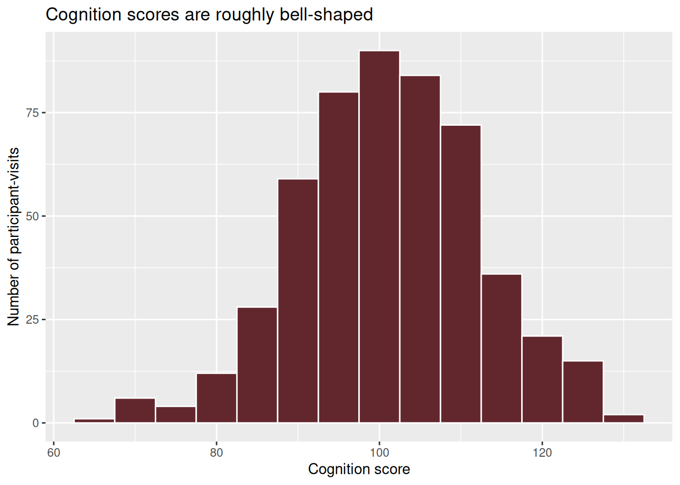
Histogram of cognition scores, roughly bell-shaped and centred near 100. — Figure 1: Distribution of cognition scores across all visits

Note the pipe carries the data in, and then layers are added with +. Mixing the two up — writing |> between layers — is the most common ggplot2 error there is.

A boxplot: comparing groups

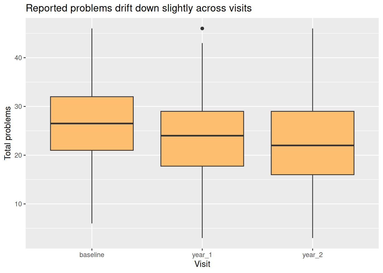
abcd |> 
  ggplot(aes(x = visit, y = total_problems)) +
  geom_boxplot(fill = "#FDBF6F") +
  labs(
    title = "Reported problems drift down slightly across visits",
    x     = "Visit",
    y     = "Total problems"
  )

Boxplots of total problem scores at baseline, year 1 and year 2, with slightly lower medians at later visits. — Figure 2: Total problems by visit

A line chart: change over time

For a trend you first have to compute the trend — one number per visit — and then plot it. Which is the group_by() + summarise() pattern from section 7, piped straight into a plot:

abcd |> 
  group_by(visit) |> 
  summarise(mean_cog = mean(cognition_score, na.rm = TRUE)) |> 
  ggplot(aes(x = visit, y = mean_cog, group = 1)) +
  geom_line(colour = "#62272D", linewidth = 1) +
  geom_point(size = 3, colour = "#62272D") +
  labs(
    title = "Mean cognition score rises across visits",
    x     = "Visit",
    y     = "Mean cognition score"
  )

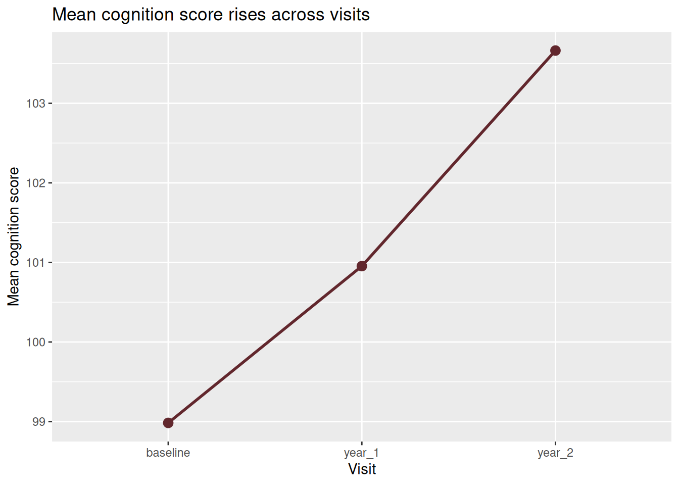
Line chart with points showing mean cognition score rising modestly from baseline through year 2. — Figure 3: Mean cognition score at each visit

group = 1 looks odd. visit is text, not a number, so ggplot2 does not know which points to join up; group = 1 says “these all belong to one line”. You will need it every time you draw a line over a categorical x-axis.

Exercise 1.5

Draw a boxplot of sleep_hrs by visit. Then add colour = sex inside aes() and see what changes.

Solution

abcd |> 
  ggplot(aes(x = visit, y = sleep_hrs, colour = sex)) +
  geom_boxplot() +
  labs(x = "Visit", y = "Sleep (hours/night)")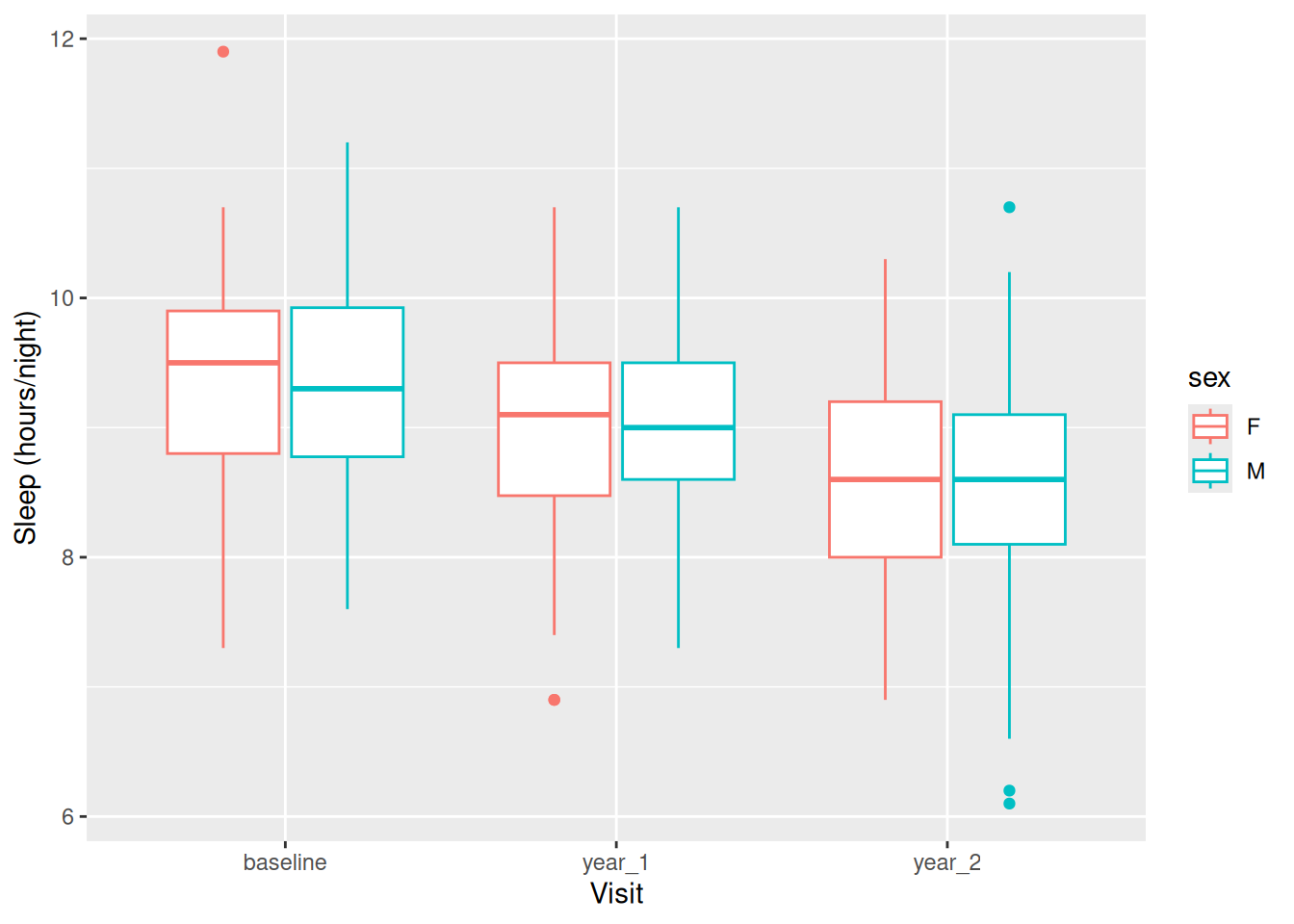

Boxplots of sleep hours by visit, split by sex.

Mapping a column to colour splits each box in two and adds a legend automatically. That is the pattern for “show me this broken down by group”.

Going deeper

More geoms, faceting into small multiples, and how to make a figure that would pass in a paper are in the plot gallery. Module 2 is devoted to this.

10. Saving your work

A result that only exists in your Console is not a result. write_csv() puts a table on disk:

visit_summary <- abcd |> 
  group_by(visit) |> 
  summarise(
    n        = n(),
    mean_cog = mean(cognition_score, na.rm = TRUE),
    mean_probs = mean(total_problems, na.rm = TRUE)
  )

write_csv(visit_summary, "output/visit-summary.csv")

And ggsave() saves the most recent plot:

ggsave("output/cognition-by-visit.png", width = 6, height = 4, dpi = 300)

This is why Module 0 had you make an output/ folder. Keeping saved results separate from raw data means you can always delete everything in output/ and rebuild it by re-running the script — which is a decent working definition of a reproducible analysis.

Putting it together

Everything from today, as one pipeline — read, clean, summarise, save:

abcd |> 
  filter(visit == "baseline") |> 
  drop_na(cognition_score) |> 
  mutate(age_years = age_months / 12) |> 
  group_by(sex) |> 
  summarise(
    n            = n(),
    mean_age     = round(mean(age_years), 1),
    mean_cog     = round(mean(cognition_score), 1),
    mean_screen  = round(mean(screen_time_hrs, na.rm = TRUE), 1)
  )

# A tibble: 2 × 5
  sex       n mean_age mean_cog mean_screen
  <chr> <int>    <dbl>    <dbl>       <dbl>
1 F        86      9.8     98.9         2.3
2 M        92      9.9     99           2.4

Read it as one sentence: take the data, keep baseline visits, drop rows missing a cognition score, add an age-in-years column, split by sex, and report these four numbers.

Two hours ago that was an opaque wall of symbols.

What you can now do

Run code from a script, and store results with <-
Read function calls, c(), $ and library() when you meet them
Load a CSV and inspect it before trusting it
Chain steps with |>
filter(), select(), arrange(), mutate(), group_by() + summarise()
Spot missing data, count it, and decide about it deliberately
Build histograms, boxplots and line charts, and save them

Recording

The following recording is of the live workshop hosted on Sep 10th, 2026.

Warning

The topics covered during the live session is a smaller subset of all the materials displayed above. We highly recommend you go through this entire page and the exercises to get comfortable with the contents / topics of Module 1.

Going further

Optional, and none of it is assumed in Module 2:

Data types deep-dive — coercion and factors in detail
Plot gallery — more geoms and faceting
R for Data Science, chapters 1–4 — the same ground, at book length
The dplyr cheatsheet — one page, keep it next to you

Next: Module 2 · Data Exploration & Visualization → on Sep 24, where the pipelines get longer and the plots get good.

1. How code gets run

Storing things: <-

2. The base R notation you need to read code

Functions and their arguments

c() — making a vector

$ — pulling one column out of a table

library() — switching a package on

3. Data types

4. Reading in the data

5. Looking at what you loaded

6. The pipe: |>

7. The five verbs that do the work

filter() — keep some rows

select() — keep some columns

arrange() — sort the rows

mutate() — add or change a column

summarise() — collapse to a single row

8. Missing data

How much is missing?

Dropping rows

9. Your first plots

A histogram: the shape of one variable

A boxplot: comparing groups

A line chart: change over time

10. Saving your work

Putting it together

What you can now do

Recording

Going further

Storing things: `<-`

`c()` — making a vector

`$` — pulling one column out of a table

`library()` — switching a package on

6. The pipe: `|>`

`filter()` — keep some rows

`select()` — keep some columns

`arrange()` — sort the rows

`mutate()` — add or change a column

`summarise()` — collapse to a single row